An analysis focused on the world university rankings published by Times Higher Education (THE) in 2023 using the R programming language…
R
Data Analysis
Data Visualization
Author
Rebekah Chuang
Published
October 17, 2023
Introduction
This dataset pertains to the world university rankings in 2023, as evaluated by Times Higher Education. The dataset has been sourced from Kaggle and contains a total of 2361 columns and 2341 rows.
While the dataset is quite extensive with 2361 columns, not all of them are pertinent for our analysis. We will address this issue during the data cleaning process. For now, let’s focus on the columns that are of particular interest:
Number of Students: The count of full-time equivalent students at the university.
Students per Staff Ratio: The ratio of full-time equivalent students to the number of academic staff, including those involved in teaching or research.
International Students Percentage: The percentage of students originating from countries outside the university’s host country.
Teaching Score: Score related to the quality of teaching.
Research Score: Score related to research quality.
Citations Score: Score related to the number of citations received.
Industry Income Score: Score associated with income generated from industry collaborations.
International Outlook Score: A score reflecting the university’s international outlook.
Female Student Ratio: The proportion of female students at the university.
Male Student Ratio: The proportion of male students at the university.
Minimum Overall Score: The lowest overall score recorded.
Maximum Overall Score: The highest overall score recorded.
University Rank: The university’s ranking, with specific rankings for institutions in the top 200, and a ranking range for those beyond the top 200.
For detailed information about how Times Higher Education evaluates universities, you can refer to their official website.
Preparation and Data Cleaning
Import Library
Code
library(tidyverse)
── Attaching core tidyverse packages ──────────────────────── tidyverse 2.0.0 ──
✔ dplyr     1.1.3     ✔ readr     2.1.4
✔ forcats   1.0.0     ✔ stringr   1.5.0
✔ ggplot2   3.4.4     ✔ tibble    3.2.1
✔ lubridate 1.9.2     ✔ tidyr     1.3.0
✔ purrr     1.0.2
── Conflicts ────────────────────────────────────────── tidyverse_conflicts() ──
✖ dplyr::filter() masks stats::filter()
✖ dplyr::lag()    masks stats::lag()
ℹ Use the conflicted package (<http://conflicted.r-lib.org/>) to force all conflicts to become errors
Code
library(ggplot2)library(plotly)
Attaching package: 'plotly'

The following object is masked from 'package:ggplot2':

    last_plot

The following object is masked from 'package:stats':

    filter

The following object is masked from 'package:graphics':

    layout
Code
library(dplyr)library(fmsb)
Import Dataset
Code
university =read_csv("Preprocessed World University Rankings 2023 Dataset.csv",show_col_types =FALSE)university
# A tibble: 2,341 × 2,362
   `No of student` `No of student per staff` `International Student`
             <dbl>                     <dbl>                   <dbl>
 1           20965                      10.6                    0.42
 2           21887                       9.6                    0.25
 3           20185                      11.3                    0.39
 4           16164                       7.1                    0.24
 5           11415                       8.2                    0.33
 6            2237                       6.2                    0.34
 7            8279                       8                      0.23
 8           40921                      18.4                    0.24
 9           13482                       5.9                    0.21
10           18545                      11.2                    0.61
# ℹ 2,331 more rows
# ℹ 2,359 more variables: `Teaching Score` <dbl>, `Research Score` <dbl>,
#   `Citations Score` <dbl>, `Industry Income Score` <dbl>,
#   `International Outlook Score` <dbl>, `Female Ratio` <dbl>,
#   `Male Ratio` <dbl>, `OverAll Score Min` <dbl>, `OverAll Score Max` <dbl>,
#   `Name of University_AGH University of Krakow` <dbl>,
#   `Name of University_Aalborg University` <dbl>, …
Show total rows and columns
Code
nrow(university) # number of rows
[1] 2341
Code
ncol(university) # number of cols
[1] 2362
When we check the number of rows and columns, there are 2341 rows and 2362 columns in this dataset, which is highly unusual, as it’s practically impossible for a university to be evaluated based on over 2,000 features in the real world. Let’s retrieve all the column names to see what’s happening.
Get all column names
Since there are 2362 columns in total, we are only showing the first 20 columns to see if we can find something.
Code
columns =colnames(university)columns[0:20]
 [1] "No of student"
 [2] "No of student per staff"
 [3] "International Student"
 [4] "Teaching Score"
 [5] "Research Score"
 [6] "Citations Score"
 [7] "Industry Income Score"
 [8] "International Outlook Score"
 [9] "Female Ratio"
[10] "Male Ratio"
[11] "OverAll Score Min"
[12] "OverAll Score Max"
[13] "Name of University_AGH University of Krakow"
[14] "Name of University_Aalborg University"
[15] "Name of University_Aalto University"
[16] "Name of University_Aarhus University"
[17] "Name of University_Abdelmalek Essaâdi University"
[18] "Name of University_Abdul Wali Khan University Mardan"
[19] "Name of University_Abdullah Gül University"
[20] "Name of University_Abertay University"
As we can see in the result, starting from column 13, all the columns provide a One Hot Encoder column to check the name of the university. For example, in the column name of University_AGH University of Krakow, if the university name for that row is AGH University of Krakow, the value should be 1; otherwise, the value is 0.
Although we didn’t show all the column names here, if you take a look at the dataset, you would find out that the same situation occurs in the Location column.
Create University Name and Location column
Now, we are going to create the University Name and Location columns to save their actual names as values. First, we’ll create a new column named University Name and check the existing column names. If a column name starts with “Name of University_” and the value in that row is 1, we’ll save the name after the underscore (_) as the university name. The same method will be applied to Location.
Check the number of unique value for University Name
Let’s take a look at how many universities are involved in this world ranking dataset!
Code
length(unique(university$`University Name`))
[1] 2234
When we check the number of unique values for University Name column, we find that there are 2234 unique universities. However, the total number of rows in this university dataset is 2341. There are two possible reasons why the number of unique universities does not equal the number of records:
Duplicate Data: Some records may be duplicates for the same university. For example, there are ten rows representing data for Harvard University.
Unknown Data: Many rows might have missing values in the University Name column, or the data collectors might have used Unknown or No Record as values in this column, and retained these rows.
How can we check and solve the problem?
We can use count() to calculate the frequency of each university appearing in the dataset.
Code
university_count = university %>%count(`University Name`) %>%arrange(desc(n))university_count
# A tibble: 2,234 × 2
   `University Name`                     n
   <chr>                             <int>
 1 Unknown University                  108
 2 AGH University of Krakow              1
 3 Aalborg University                    1
 4 Aalto University                      1
 5 Aarhus University                     1
 6 Abdelmalek Essaâdi University         1
 7 Abdul Wali Khan University Mardan     1
 8 Abdullah Gül University               1
 9 Abertay University                    1
10 Aberystwyth University                1
# ℹ 2,224 more rows
After counting the frequency of each university appearing in the dataset and sorting the data by frequency in descending order, it turns out that there are 108Unknown University entries. This analysis shows that the existence of unknown data is the reason why the number of rows doesn’t match the number of unique universities.
Remove university with unknown name
This analysis pertains to world universities ranking, and it would make no sense if we do not know which university we are referring to. Therefore, it is essential that we remove those rows with unknown values.
Code
university_updated = university %>%filter(`University Name`!="Unknown University")university_updated
# A tibble: 0 × 15
# ℹ 15 variables: No of student <dbl>, No of student per staff <dbl>,
#   International Student <dbl>, Teaching Score <dbl>, Research Score <dbl>,
#   Citations Score <dbl>, Industry Income Score <dbl>,
#   International Outlook Score <dbl>, Female Ratio <dbl>, Male Ratio <dbl>,
#   OverAll Score Min <dbl>, OverAll Score Max <dbl>, University Rank <chr>,
#   University Name <chr>, Location <chr>
Although we have already removed the rows where University Name equals Unknown University, we haven’t checked for any NA values in the column.
Code
sum(is.na(university_updated$`University Name`))
[1] 0
After checking, we found that there is no row containing NA in the University Name.
Check University Rank column
For this analysis, we are only focusing on universities that have a ranking. Let’s look at the University Rank column!
# A tibble: 100 × 2
   Location             n
   <chr>            <int>
 1 United States      171
 2 Unknown Location   151
 3 Japan              115
 4 United Kingdom      89
 5 China               82
 6 India               65
 7 Brazil              62
 8 Iran                61
 9 Turkey              56
10 Spain               54
# ℹ 90 more rows
As we can see in the result, there are 151 universities without location, let’s take a look at those universities.
# A tibble: 151 × 3
   `University Rank` `University Name`                Location
   <chr>             <chr>                            <chr>
 1 16                Tsinghua University              Unknown Location
 2 17                Peking University                Unknown Location
 3 19                National University of Singapore Unknown Location
 4 30                Technical University of Munich   Unknown Location
 5 31                University of Hong Kong          Unknown Location
 6 33                LMU Munich                       Unknown Location
 7 42                KU Leuven                        Unknown Location
 8 43                Universität Heidelberg           Unknown Location
 9 45                Chinese University of Hong Kong  Unknown Location
10 46                McGill University                Unknown Location
# ℹ 141 more rows
If you take a look at those universities, you will find that most of them are prestigious institutions with excellent rankings. Removing all of them might significantly impact our analysis. Therefore, the best way to address this problem is to manually update their locations.
NOTE: This may not be a practical method for other datasets, as they often contain hundreds of thousands of missing data, making it too time-consuming to correct them all manually.
Code
university_all <- university_updated %>%mutate(Location =case_when(`University Name`=="Tsinghua University"~"China",`University Name`=="Peking University"~"China",`University Name`=="National University of Singapore"~"Singapore",`University Name`=="Technical University of Munich"~"Germany",`University Name`=="University of Hong Kong"~"Hong Kong",`University Name`=="LMU Munich"~"Germany",`University Name`=="KU Leuven"~"Belgium",`University Name`=="Universität Heidelberg"~"Germany",`University Name`=="Chinese University of Hong Kong"~"Hong Kong",`University Name`=="McGill University"~"Canada",`University Name`=="The University of Queensland"~"Australia",`University Name`=="University of Manchester"~"United Kingdom",`University Name`=="The Hong Kong University of Science and Technology"~"Hong Kong",`University Name`=="Zhejiang University"~"China",`University Name`=="UNSW Sydney"~"Australia",`University Name`=="University of Science and Technology of China"~"China",`University Name`=="University of Groningen"~"Netherlands",`University Name`=="University of Bristol"~"United Kingdom",`University Name`=="Leiden University"~"Netherlands",`University Name`=="Yonsei University (Seoul campus)"~"South Korea",`University Name`=="Hong Kong Polytechnic University"~"Hong Kong",`University Name`=="Erasmus University Rotterdam"~"Netherlands",`University Name`=="University of Glasgow"~"United Kingdom",`University Name`=="McMaster University"~"Canada",`University Name`=="University of Adelaide"~"Australia",`University Name`=="City University of Hong Kong"~"Hong Kong",`University Name`=="King Abdulaziz University"~"Saudi Arabia",`University Name`=="University of Warwick"~"United Kingdom",`University Name`=="University of Montreal"~"Canada",`University Name`=="Université Paris Cité"~"France",`University Name`=="University of Sheffield"~"United Kingdom",`University Name`=="University of Technology Sydney"~"Australia",`University Name`=="University of Ottawa"~"Canada",`University Name`=="Newcastle University"~"United Kingdom",`University Name`=="Radboud University Nijmegen"~"Netherlands",`University Name`=="Arizona State University (Tempe)"~"Netherlands",`University Name`=="University of Cape Town"~"South Africa",`University Name`=="University of Bologna"~"Italy",`University Name`=="Trinity College Dublin"~"Ireland",`University Name`=="Pohang University of Science and Technology (POSTECH)"~"South Korea",`University Name`=="Southern University of Science and Technology (SUSTech)"~"China",`University Name`=="Sungkyunkwan University (SKKU)"~"South Korea",`University Name`=="Ulsan National Institute of Science and Technology (UNIST)"~"South Korea",`University Name`=="University of Liverpool"~"United Kingdom",`University Name`=="Cardiff University"~"United Kingdom",`University Name`=="National Taiwan University (NTU)"~"Taiwan",`University Name`=="Queen’s University Belfast"~"United Kingdom",`University Name`=="Curtin University"~"United Kingdom",`University Name`=="University of East Anglia"~"United Kingdom",`University Name`=="Humanitas University"~"Italy",`University Name`=="Korea University"~"South Korea",`University Name`=="University of Macau"~"China",`University Name`=="Macau University of Science and Technology"~"China",`University Name`=="Queensland University of Technology"~"Australia",`University Name`=="RCSI University of Medicine and Health Sciences"~"Ireland",`University Name`=="Sant’Anna School of Advanced Studies – Pisa"~"Italy",`University Name`=="Semmelweis University"~"Hungary",`University Name`=="University of Tartu"~"Estonia",`University Name`=="Western University"~"Canada",`University Name`=="Auckland University of Technology"~"New Zealand",`University Name`=="Griffith University"~"Australia",`University Name`=="Kyung Hee University"~"South Korea",`University Name`=="La Trobe University"~"Australia",`University Name`=="Queen’s University"~"Canada",`University Name`=="Simon Fraser University"~"Canada",`University Name`=="Stellenbosch University"~"South Africa",`University Name`=="Tilburg University"~"Netherlands",`University Name`=="United Arab Emirates University"~"United Arab Emirates",`University Name`=="Virginia Polytechnic Institute and State University"~"United States",`University Name`=="University of the Witwatersrand"~"South Africa",`University Name`=="Alfaisal University"~"Saudi Arabia",`University Name`=="University of Bordeaux"~"France",`University Name`=="Dalhousie University"~"Canada",`University Name`=="University of Oulu"~"Finland",`University Name`=="Politecnico di Milano"~"Italy",`University Name`=="University of South Australia"~"Australia",`University Name`=="Taipei Medical University"~"Taiwan",`University Name`=="University of Cape Coast"~"Ghana",`University Name`=="Edith Cowan University"~"Australia",`University Name`=="Khalifa University"~"United Arab Emirates",`University Name`=="University of Turku"~"Finland",`University Name`=="University of Cyprus"~"Cyprus",`University Name`=="Hanyang University"~"South Korea",`University Name`=="University of KwaZulu-Natal"~"South Africa",`University Name`=="Sabancı University"~"Turkey",`University Name`=="Southern Medical University"~"China",`University Name`=="Ton Duc Thang University"~"Vietnam",`University Name`=="York University"~"Canada",`University Name`=="An-Najah National University"~"Palestine",`University Name`=="Constructor University Bremen"~"Germany",`University Name`=="University of Nicosia"~"Cyprus",`University Name`=="Saveetha Institute of Medical and Technical Sciences"~"India",`University Name`=="University of Canterbury"~"New Zealand",`University Name`=="Central Queensland University"~"Australia",`University Name`=="Chongqing University"~"China",`University Name`=="Covenant University"~"Nigeria",`University Name`=="Eötvös Loránd University"~"Hungary",`University Name`=="Federation University Australia"~"Australia",`University Name`=="Graphic Era University"~"India",`University Name`=="University of Johannesburg"~"South Africa",`University Name`=="KIIT University"~"India",`University Name`=="University of Limerick"~"Ireland",`University Name`=="Maharishi Markandeshwar University (MMU)"~"India",`University Name`=="Memorial University of Newfoundland"~"Canada",`University Name`=="National Cheng Kung University (NCKU)"~"Taiwan",`University Name`=="Soochow University, China"~"China",`University Name`=="Chengdu University"~"China",`University Name`=="Chulalongkorn University"~"Thailand",`University Name`=="Coventry University"~"United Kingdom",`University Name`=="Kuwait University"~"Kuwait",`University Name`=="Kyungpook National University"~"South Korea",`University Name`=="Lovely Professional University"~"India",`University Name`=="Monterrey Institute of Technology"~"Mexico",`University Name`=="National Taiwan Normal University"~"Taiwan",`University Name`=="Symbiosis International University"~"India",`University Name`=="Toronto Metropolitan University"~"Canada",`University Name`=="Atılım University"~"Turkey",`University Name`=="University of Calcutta"~"India",`University Name`=="Carlos III University of Madrid"~"Spain",`University Name`=="Chang Gung University"~"Taiwan",`University Name`=="Chonnam National University"~"South Korea",`University Name`=="University of Debrecen"~"Hungary",`University Name`=="University of Indonesia"~"Indonesia",`University Name`=="Jeonbuk National University"~"South Korea",`University Name`=="Jiangnan University"~"China",`University Name`=="Pusan National University"~"South Korea",`University Name`=="Siksha ‘O’ Anusandhan"~"India",`University Name`=="Tokyo Metropolitan University"~"Japan",`University Name`=="Yıldız Technical University"~"Turkey",`University Name`=="Acıbadem University"~"Turkey",`University Name`=="Universitas Airlangga"~"Indonesia",`University Name`=="The Catholic University of Korea"~"South Korea",`University Name`=="Chungbuk National University"~"South Korea",`University Name`=="De La Salle University"~"Philippines",`University Name`=="Gyeongsang National University"~"South Korea",`University Name`=="The Hashemite University"~"Jordan",`University Name`=="Istanbul Medipol University"~"Turkey",`University Name`=="Jeju National University"~"South Korea",`University Name`=="Kangwon National University"~"South Korea",`University Name`=="Universiti Malaysia Sarawak (UNIMAS)"~"Malaysia",`University Name`=="National Chung Cheng University"~"Taiwan",`University Name`=="National Dong Hwa University"~"Taiwan",`University Name`=="Qassim University"~"Saudi Arabia",`University Name`=="Sathyabama Institute of Science and Technology"~"India",`University Name`=="Southwest Jiaotong University"~"China",`University Name`=="Thammasat University"~"Thailand",`University Name`=="Burapha University"~"Thailand",`University Name`=="University of Guadalajara"~"Mexico",`University Name`=="Mapúa University"~"Philippines",`University Name`=="Sophia University"~"Japan",`University Name`=="VSB - Technical University of Ostrava"~"Czech Republic",TRUE~ Location # Keep other values unchanged ))university_all
After using glimpse(university_all) to inspect the data types of all columns, we observe a small issue in the No of student column. The data type for this column is listed as dbl, but the number of students should always be an integer. Therefore, we need to rectify this by changing the data type to integer.
NOTE: For the University Ranking columns, although the ranking should be an integer as well, this dataset sets the ranking for universities out of 200 as a range (e.g., 201-250). We cannot directly turn them into integers now, but we will deal with this problem later.
Code
university_all$`No of student`<-as.integer(university_all$`No of student`)
Let’s check again if the datatype for No of student column has been changed!
If we revisit the analysis conducted earlier, we know that there are a total of 101 different locations (countries) with universities in this world university ranking. Now, let’s determine which country has the highest number of universities.
In the following section, I will create a bar chart that displays countries with at least 30 universities listed, and sort the results in descending order. As the result shown below, there are 17 countries with at least 30 universities listed.
# A tibble: 17 × 2
   Location           n
   <chr>          <int>
 1 United States    172
 2 Japan            117
 3 United Kingdom   101
 4 China             95
 5 India             74
 6 Brazil            62
 7 Iran              61
 8 Turkey            61
 9 Italy             55
10 Spain             55
11 Germany           48
12 Taiwan            43
13 France            42
14 Australia         36
15 South Korea       36
16 Poland            32
17 Canada            30
Since I will be creating the same location frequency plot with different data sources, I’m writing the plot into a function so that it can be reused.
Code
create_location_plot <-function(data) { location_plot <-ggplot(data, aes(x = n, y =reorder(Location, n))) +geom_bar(stat ="identity", fill ="#A39183") +labs(title ="Number of Universities from Each Country on the Ranking List",x ="Counts",y ="" ) location_plot <- location_plot +aes(text =paste("Number of Universities: ", n, "")) +theme(plot.title =element_text(hjust =0.5) )return(ggplotly(location_plot, tooltip ="text"))}
However, this dataset contains rankings from 1 to over 1500. It would be more realistic to focus on the top 200 universities’ locations and determine which country has more prestigious universities in their area.
Code
# replace any non-numeric characters to "" and convert to numerictop_200_university <- university_all %>%mutate(`University Rank`=as.numeric(gsub("[^0-9]", "", `University Rank`)))# Filter out universities not in the top 200top_200_university <- top_200_university %>%filter(`University Rank`<=200)top_200_university
# A tibble: 26 × 2
   Location           n
   <chr>          <int>
 1 United States     57
 2 United Kingdom    28
 3 Germany           22
 4 China             11
 5 Netherlands       11
 6 Australia         10
 7 Canada             7
 8 South Korea        6
 9 Switzerland        6
10 France             5
# ℹ 16 more rows
In today’s world, the right to education is more equitable than it used to be. It is crucial to ensure that there is no gender bias when evaluating university applications. Let’s examine the average female-to-male ratio in the top 200 universities in each country!
# A tibble: 26 × 2
   Location  `Average Gender Ratio`
   <chr>                      <dbl>
 1 Australia                  5.4
 2 Austria                   12.7
 3 Belgium                    9
 4 Canada                    10.5
 5 China                      0.863
 6 Denmark                   -0.667
 7 Finland                   34
 8 France                    -0.8
 9 Germany                    1.20
10 Hong Kong                  4.27
# ℹ 16 more rows
Code
gender_ratio_plot =ggplot(top_200_university_gender_ratio,aes(x =`Average Gender Ratio`,y =`Location`,text =paste("Average F-M Gender Ratio(%):", round(`Average Gender Ratio`, 2), "%","\nLocation:", `Location`, ""))) +geom_bar(stat ="identity",aes(fill =ifelse(`Average Gender Ratio`<0, "Female < Male", "Female > Male"))) +scale_fill_manual(values =c("Female < Male"="#0072B2", "Female > Male"="#E69F00")) +labs(x ="Average Gender Ratio", y ="Location") +ggtitle("Average Gender Ratio by Country for Top 200 Universities") +labs(fill ="Gender Ratio")gender_ratio_plot = gender_ratio_plot +theme(plot.title =element_text(hjust =0.5))ggplotly(gender_ratio_plot, tooltip ="text")
As we can see from the bar plot above, when considering the top 200 universities, more countries have a higher average female-to-male ratio.
Relationship & Correlation
In this dataset, we can see that there are many features that determine whether a university’s overall score is high, which makes it have a good ranking. These features include the number of students, the number of students per staff, the international student ratio, the teaching score, the research score, the citations score, the industry income score, and the international outlook score. However, not every feature will be related to the final score. In the following part, I’ll use two different methods to determine the correlation between each feature and the overall score:
Scatter Plot
Calculating Correlation Coefficients: While visual inspection through a scatter plot is one way to assess linearity, calculating the correlation coefficient provides a more quantitative measure:
A correlation coefficient near 0 suggests a weak linear relationship.
A correlation coefficient near 1 indicates a strong positive linear relationship.
A correlation coefficient near -1 indicates a strong negative linear relationship.
First, let’s create a function to generate scatter plots so that we can reuse it in the following plots:
Relationship between Number of Student & Overall Score
Code
create_scatter_plot(top_200_university, top_200_university$`No of student`, "Number of Student")
After analyzing the scatter plot that illustrates the relationship between a university’s score and the number of students, it appears that there is no strong correlation between these two features. However, a more precise assessment can be made by calculating correlation coefficients.
Code
coefficient =cor.test(top_200_university$`No of student`, top_200_university$`OverAll Score Max`)coefficient$estimate
        cor
0.007483786
Based on this analysis, the sample estimate of the correlation coefficient is 0.007483786, which is very close to 0. This suggests that there is no strong evidence of a linear correlation between the number of students and the overall score in the data.
Relationship between Number of Student per Staff & Overall Score
Code
create_scatter_plot(top_200_university, top_200_university$`No of student per staff`, "Number of Student per Staff")
Code
coefficient =cor.test(top_200_university$`No of student per staff`, top_200_university$`OverAll Score Max`)coefficient$estimate
       cor
-0.2354278
Based on this analysis, the sample estimate of the correlation coefficient is -0.2354278, this suggests that as the number of students per staff increases, the overall score tends to decrease, but the relationship is not very strong.
Relationship between International Student Ratio & Overall Score
Based on this analysis, the sample estimate of the correlation coefficient is 0.334458, which is moderately close to 1. This suggests that there is a moderate positive linear correlation between international student ratio and the overall score in the data.
Relationship between Teaching Score & Overall Score
Based on this analysis, the sample estimate of the correlation coefficient is 0.8962569, which is very close to 1. This suggests that there is strong evidence of a significant positive linear correlation between teaching score and the overall score in the data.
Relationship between Research Score & Overall Score
Based on this analysis, the sample estimate of the correlation coefficient is 0.9299495, which is very close to 1. This suggests that there is strong evidence of a significant positive linear correlation between research score and the overall score in the data.
Relationship between Citations Score & Overall Score
Based on this analysis, the sample estimate of the correlation coefficient is 0.4195276, which is moderately close to 1. This suggests that there is a moderate positive linear correlation between citations score and the overall score in the data.
Relationship between Industry Income Score & Overall Score
Code
create_scatter_plot(top_200_university, top_200_university$`Industry Income Score`, "Industry Income Score")
Code
coefficient =cor.test(top_200_university$`Industry Income Score`, top_200_university$`OverAll Score Max`)coefficient$estimate
      cor
0.1866167
Based on this analysis, the sample estimate of the correlation coefficient is 0.1866167, this suggests that as industry income score increases, the overall score also tends to increase, but the relationship is not very strong.
Relationship between International Outlook Score & Overall Score
Code
create_scatter_plot(top_200_university, top_200_university$`International Outlook Score`, "International Outlook Score")
Code
coefficient =cor.test(top_200_university$`International Outlook Score`, top_200_university$`OverAll Score Max`)coefficient$estimate
      cor
0.2104629
Based on this analysis, the sample estimate of the correlation coefficient is 0.2104629,this suggests that as international outlook score increases, the overall score also tends to increase, but the relationship is not very strong.
Based on this analysis, the sample estimate of the correlation coefficient is -0.0912758, which is very close to 0. This suggests that there is no strong evidence of a linear correlation between female ratio and the overall score in the data.
Based on this analysis, the sample estimate of the correlation coefficient is 0.0912758, which is very close to 0. This suggests that there is no strong evidence of a linear correlation between male ratio and the overall score in the data.
How do the top 10 universities in the world perform?
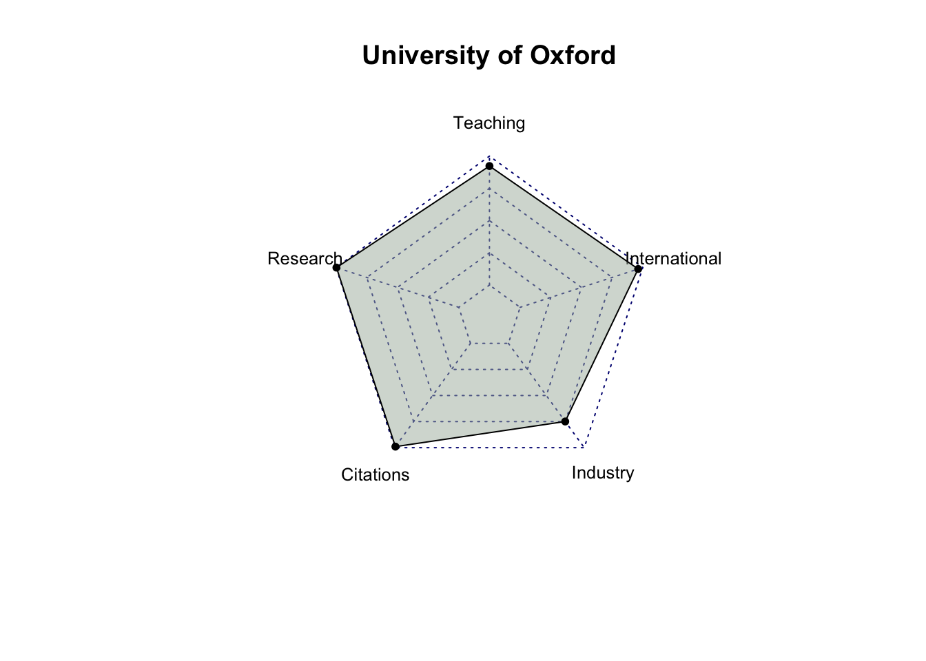
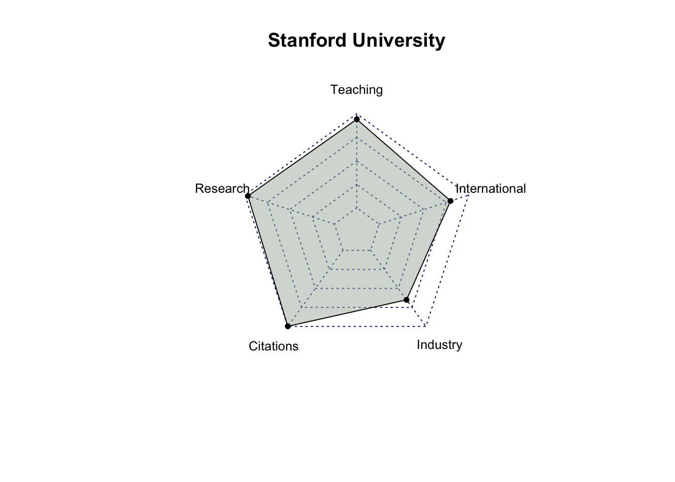
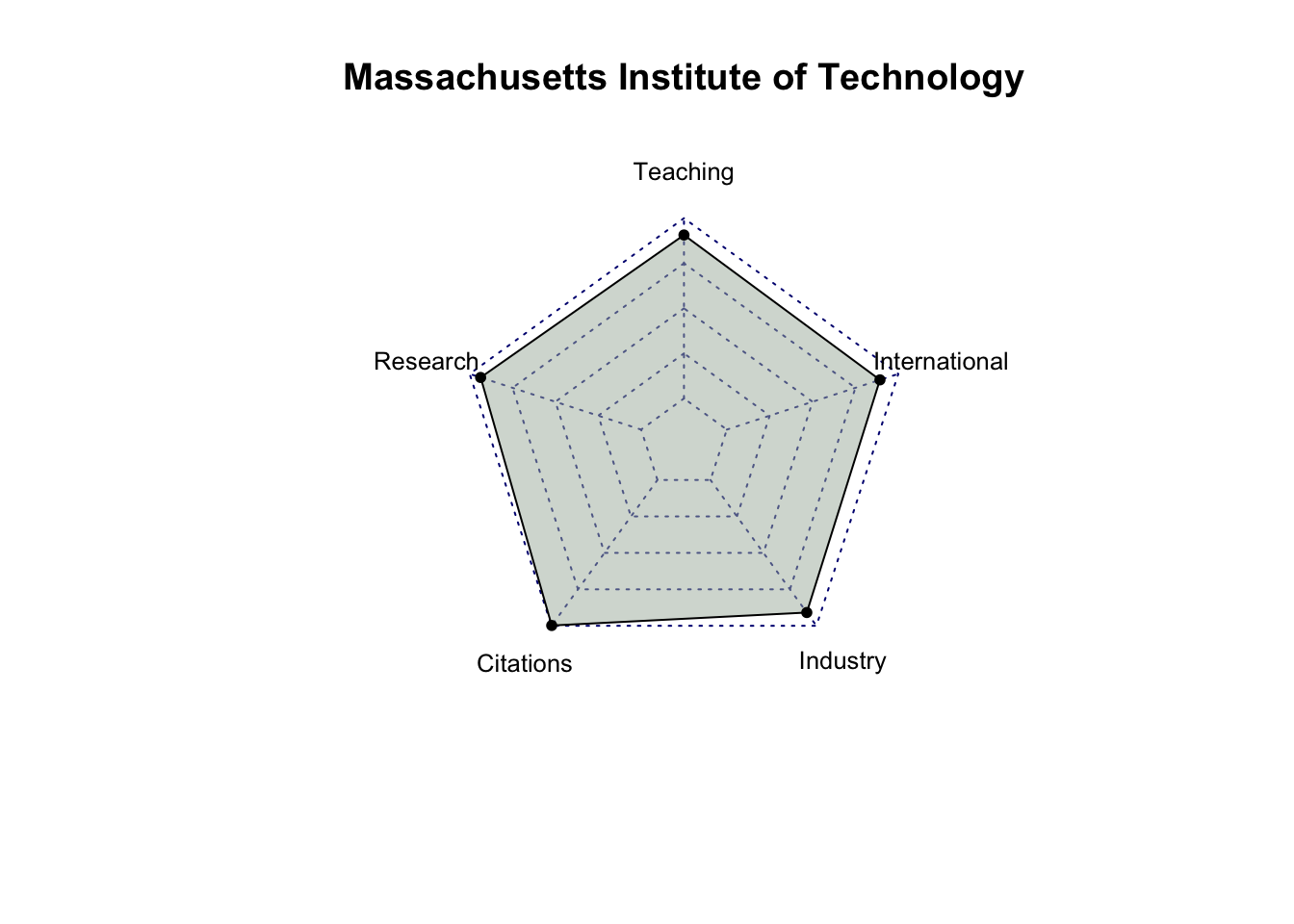
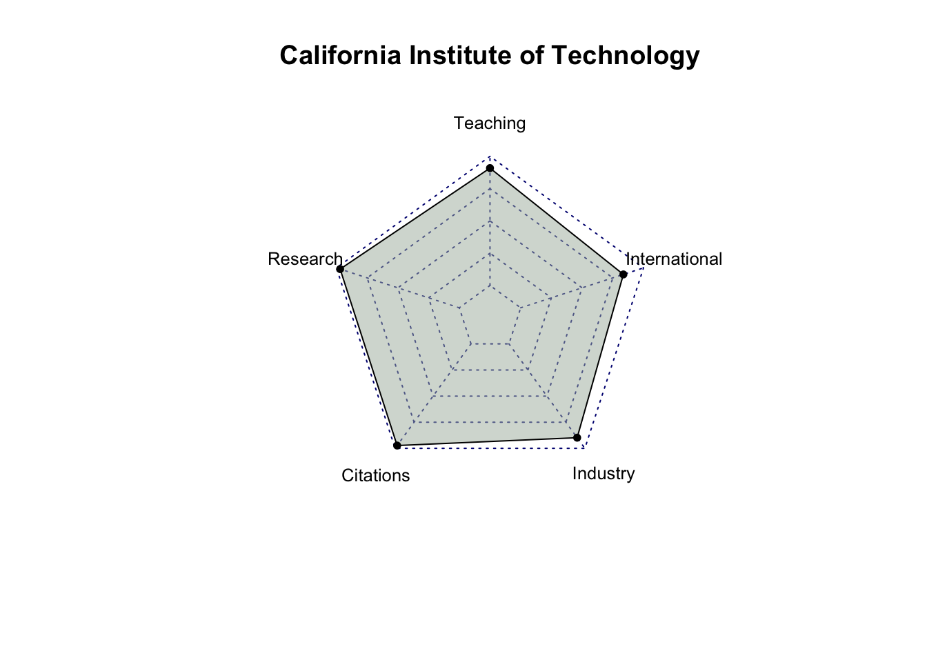
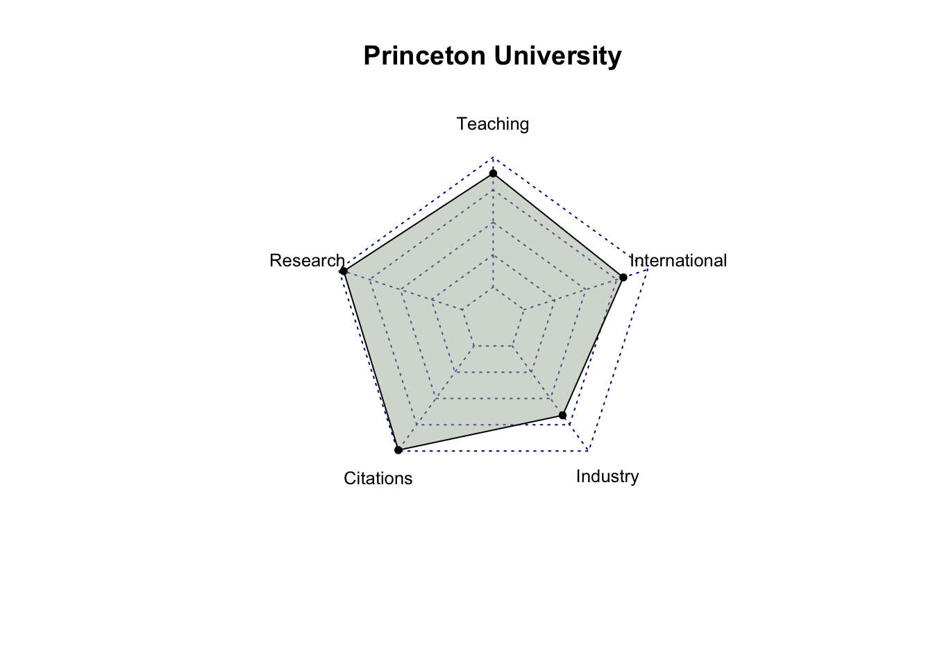
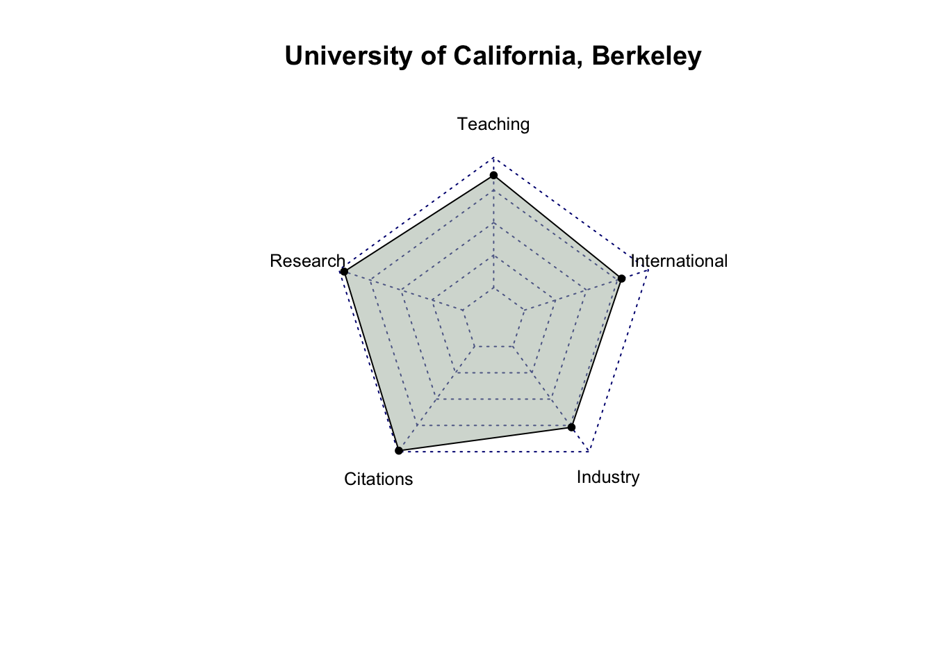
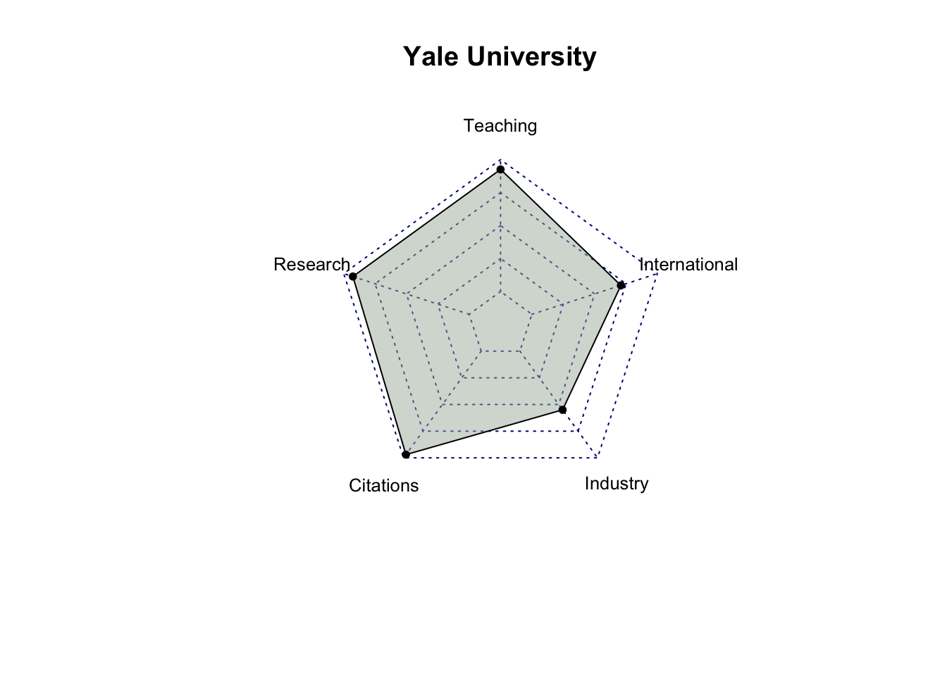
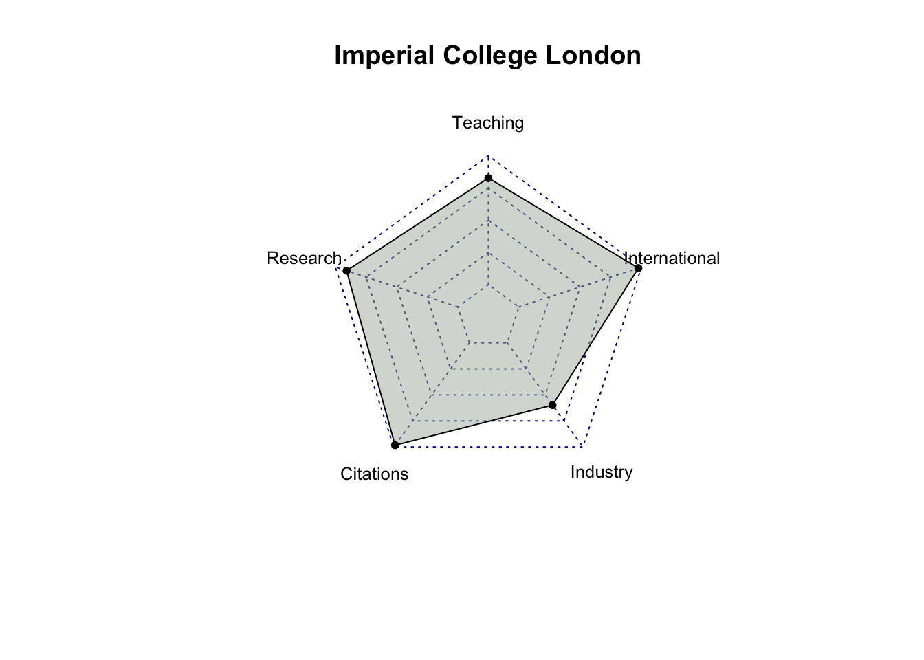
In the dataset, we can see that there are five columns related to scores, including teaching score, research score, citations score, industry income score, and international outlook score. It’s no doubt that the top 10 universities have perfect scores in all of these features, but it’s also worthwhile to examine how these universities perform in these areas or which aspect they focus on the most.
We are going to prepare data for the top 10 universities and create a radar chart for each of them.
Code
# select only score related columns and university namescore_data = top_200_university %>%select(`University Name`, `Teaching Score`, `Research Score`,`Citations Score`, `Industry Income Score`, `International Outlook Score`) %>%head(10)# turn score_data into a data framescore_data =as.data.frame(score_data)# set university name as indexrownames(score_data) = score_data$`University Name`# remove the original column for university name and rename the other columnsscore_data = score_data %>%select(`Teaching Score`, `Research Score`, `Citations Score`, `Industry Income Score`, `International Outlook Score`) %>%rename(Teaching =`Teaching Score`,Research =`Research Score`,Citations =`Citations Score`,Industry =`Industry Income Score`,International =`International Outlook Score` )score_data
                                      Teaching Research Citations Industry
University of Oxford                      92.3     99.7      99.0     74.9
Harvard University                        94.8     99.0      99.3     49.5
University of Cambridge                   90.9     99.5      97.0     54.2
Stanford University                       94.2     96.7      99.8     65.0
Massachusetts Institute of Technology     90.7     93.6      99.8     90.9
California Institute of Technology        90.9     97.0      97.3     89.8
Princeton University                      87.6     95.9      99.1     66.0
University of California, Berkeley        86.4     95.8      99.0     76.8
Yale University                           92.6     92.7      97.0     55.0
Imperial College London                   82.8     90.8      98.3     59.8
                                      International
University of Oxford                           96.2
Harvard University                             80.5
University of Cambridge                        95.8
Stanford University                            79.8
Massachusetts Institute of Technology          89.3
California Institute of Technology             83.6
Princeton University                           80.3
University of California, Berkeley             78.4
Yale University                                70.9
Imperial College London                        97.5
Code
# create radar charts for top 10 university for (i in1:10) { uni = score_data[i, ] uni =data.frame(rbind(rep(100,5) , rep(0,5) , uni))radarchart(uni,seg =4,cglty =3,pty =20,vlcex =0.8,pfcol ="#A9B7AA80")title(row.names(score_data)[i])}
After analyzing the radar charts for each university, it’s evident that, among all the attributes, industry income is the one receiving less emphasis from most universities. While MIT has relatively similar scores in Teaching, Research, Citations, and International categories, with a significantly higher score in Industry Income, it doesn’t hold the first place in the rankings. This suggests that Industry Income may be a less influential factor among these five criteria. It’s also possible that factors other than scores play a significant role in determining a university’s ranking.
Also, among the top 10 universities, Massachusetts Institute of Technology (MIT) and California Institute of Technology (Cal Tech) exhibit balanced performance across all criteria compared to the other universities.”
Multiple Linear Regression Model
Keep numerical columns:
Before building a multiple linear regression model to predict the overall score and understand what makes a university good, we need to examine the columns in the university_all data frame. We will retain only the numerical data, removing categorical columns.
After taking a look at the data frame, we will exclude the following columns: University Name (categorical data), Location (categorical data), University Rank (because universities ranked beyond the top 200 are represented as a range rather than a specific rank, and ranking is actually based on the overall score), and OverAll Score Min (since its values are the same as those in OverAll Score Max).
Code
lm_data = university_all %>%select(`OverAll Score Max`, `No of student`, `No of student per staff`, `International Student`, `Teaching Score`, `Research Score`, `Citations Score`, `Industry Income Score`, `International Outlook Score`, `Female Ratio`, `Male Ratio`)glimpse(lm_data)
One of the assumptions of creating a linear regression model is that the data is linear, although creating a scatter plot is a way to check the linearity, calculating correlation coefficient is more accurate: - A correlation coefficient near 0 suggests a weak linear relationship. - A correlation coefficient near 1 or -1 suggests a strong linear relationship.
Code
cor(lm_data, method ="pearson")
                            OverAll Score Max No of student
OverAll Score Max                  1.00000000   0.015198783
No of student                      0.01519878   1.000000000
No of student per staff           -0.03180487   0.373744220
International Student              0.56448737  -0.097230825
Teaching Score                     0.82001745  -0.001826246
Research Score                     0.87286717   0.022473884
Citations Score                    0.84952680   0.026195480
Industry Income Score              0.45324234  -0.016473515
International Outlook Score        0.65116514  -0.034050167
Female Ratio                       0.08147747   0.078017459
Male Ratio                        -0.08147747  -0.078017459
                            No of student per staff International Student
OverAll Score Max                      -0.031804866            0.56448737
No of student                           0.373744220           -0.09723082
No of student per staff                 1.000000000           -0.02023569
International Student                  -0.020235693            1.00000000
Teaching Score                         -0.130568505            0.41463383
Research Score                          0.006685824            0.50729150
Citations Score                        -0.005684043            0.41098909
Industry Income Score                  -0.002587535            0.21477345
International Outlook Score             0.029469919            0.81241004
Female Ratio                            0.046239403            0.09278318
Male Ratio                             -0.046239403           -0.09278318
                            Teaching Score Research Score Citations Score
OverAll Score Max              0.820017452    0.872867170     0.849526804
No of student                 -0.001826246    0.022473884     0.026195480
No of student per staff       -0.130568505    0.006685824    -0.005684043
International Student          0.414633828    0.507291499     0.410989092
Teaching Score                 1.000000000    0.886743917     0.468045075
Research Score                 0.886743917    1.000000000     0.519222138
Citations Score                0.468045075    0.519222138     1.000000000
Industry Income Score          0.492375982    0.590539994     0.199520287
International Outlook Score    0.381143251    0.535830756     0.542363659
Female Ratio                  -0.005123603   -0.010259322     0.141017197
Male Ratio                     0.005123603    0.010259322    -0.141017197
                            Industry Income Score International Outlook Score
OverAll Score Max                     0.453242341                  0.65116514
No of student                        -0.016473515                 -0.03405017
No of student per staff              -0.002587535                  0.02946992
International Student                 0.214773454                  0.81241004
Teaching Score                        0.492375982                  0.38114325
Research Score                        0.590539994                  0.53583076
Citations Score                       0.199520287                  0.54236366
Industry Income Score                 1.000000000                  0.21562918
International Outlook Score           0.215629178                  1.00000000
Female Ratio                         -0.173404129                  0.18432870
Male Ratio                            0.173404129                 -0.18432870
                            Female Ratio   Male Ratio
OverAll Score Max            0.081477473 -0.081477473
No of student                0.078017459 -0.078017459
No of student per staff      0.046239403 -0.046239403
International Student        0.092783179 -0.092783179
Teaching Score              -0.005123603  0.005123603
Research Score              -0.010259322  0.010259322
Citations Score              0.141017197 -0.141017197
Industry Income Score       -0.173404129  0.173404129
International Outlook Score  0.184328703 -0.184328703
Female Ratio                 1.000000000 -1.000000000
Male Ratio                  -1.000000000  1.000000000
After reviewing the results, it appears that No of student, No of student per staff, Female Ratio, and Male Ratio should be removed from the lm_data because their correlation coefficients with the OverAll Score Max are pretty close to 0. This suggests that there is little to no correlation between these features and the OverAll Score Max.
Code
lm_data = university_all %>%select(`OverAll Score Max`, `International Student`, `Teaching Score`, `Research Score`, `Citations Score`, `Industry Income Score`, `International Outlook Score`)glimpse(lm_data)
model =lm(`OverAll Score Max`~`International Student`+`Teaching Score`+`Research Score`+`Citations Score`+`Industry Income Score`+`International Outlook Score`, data = lm_data)summary(model)
Call:
lm(formula = `OverAll Score Max` ~ `International Student` +
    `Teaching Score` + `Research Score` + `Citations Score` +
    `Industry Income Score` + `International Outlook Score`,
    data = lm_data)

Residuals:
    Min      1Q  Median      3Q     Max
-3.1619 -0.9467 -0.0844  0.9038  9.1780

Coefficients:
                              Estimate Std. Error t value Pr(>|t|)
(Intercept)                   4.677655   0.173290  26.993  < 2e-16 ***
`International Student`       0.160685   0.491872   0.327    0.744
`Teaching Score`              0.278230   0.005850  47.557  < 2e-16 ***
`Research Score`              0.292705   0.005436  53.847  < 2e-16 ***
`Citations Score`             0.276618   0.001590 173.955  < 2e-16 ***
`Industry Income Score`       0.015590   0.002887   5.401 7.57e-08 ***
`International Outlook Score` 0.069538   0.002969  23.423  < 2e-16 ***
---
Signif. codes:  0 '***' 0.001 '**' 0.01 '*' 0.05 '.' 0.1 ' ' 1

Residual standard error: 1.412 on 1690 degrees of freedom
Multiple R-squared:  0.9914,    Adjusted R-squared:  0.9913
F-statistic: 3.24e+04 on 6 and 1690 DF,  p-value: < 2.2e-16
After building the model and using summary() to assess its performance, we can see that the p-value for International Student is high(0.744>= 0.05), which means that the international student ratio is not statistically significant in predicting the overall score for a university. On the other hand, Teaching Score, Research Score, Citations Score, Industry Income Score, and International Outlook Score have very low p-values, indicating high significance. Let’s remove the International Student column from the model and run it again.
Code
model2 =lm(`OverAll Score Max`~`Teaching Score`+`Research Score`+`Citations Score`+`Industry Income Score`+`International Outlook Score`, data = lm_data)summary(model2)
Call:
lm(formula = `OverAll Score Max` ~ `Teaching Score` + `Research Score` +
    `Citations Score` + `Industry Income Score` + `International Outlook Score`,
    data = lm_data)

Residuals:
    Min      1Q  Median      3Q     Max
-3.1474 -0.9397 -0.0831  0.8941  9.1800

Coefficients:
                              Estimate Std. Error t value Pr(>|t|)
(Intercept)                   4.658552   0.163083  28.566  < 2e-16 ***
`Teaching Score`              0.278522   0.005780  48.185  < 2e-16 ***
`Research Score`              0.292647   0.005431  53.880  < 2e-16 ***
`Citations Score`             0.276549   0.001575 175.551  < 2e-16 ***
`Industry Income Score`       0.015577   0.002886   5.398 7.67e-08 ***
`International Outlook Score` 0.070252   0.002009  34.966  < 2e-16 ***
---
Signif. codes:  0 '***' 0.001 '**' 0.01 '*' 0.05 '.' 0.1 ' ' 1

Residual standard error: 1.412 on 1691 degrees of freedom
Multiple R-squared:  0.9914,    Adjusted R-squared:  0.9914
F-statistic: 3.889e+04 on 5 and 1691 DF,  p-value: < 2.2e-16